If you're using dates in one of your spreadsheets and you find yourself manually updating those dates then you should consider looking into the many Data and Time functions available in Excel. I'll cover some of the ones I find more useful and then provide some real world examples of how to use these functions.

Note: Some of the functions I discuss require that the *Analysis ToolPak add-in be installed. To do this in Excel, go to Tools->Add-Ins. Ensure that the Analysis ToolPak checkbox is selected. If it isn't then select it and Excel will install the Add-In.

How Excel handles dates

Excel handles dates as sequential numbers starting from January 1, 1900. Any date in excel can be converted into a 'serial number' which makes it easy to perform calculations using dates. For example, January 1, 1900 is serial number 1 and February 10, 2006 is serial number 38758.

Calculate the number of days between dates

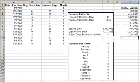
Say you have a large list of dates and you want to determine the average number of days between dates. An example might be an organization that tracks when incidents occur by logging the date of the incident. Look at Figure 1 above and you can see that there is a list of dates when incidents occurred. The second column calculates the number of days between those dates by simple use of subtraction. The formula used in cell B3 is =A3-A2 which gives a result of 24 days.

Calculate the number of business days between dates

What about business days? Excel has a function for that called NETWORKDAYS. The NETWORKDAYS function has three parameters that it will accept: start_date, end_date, and holidays. This is why I have a list of holidays in column H, it tells the NETWORKDAYS function to omit those dates as business days. The holidays parameter is optional but you must enter a start_date and an end_date. To calculate the business days the formula in C3 looks like this: =NETWORKDAYS(A2,A3,H$3:H$11) which returns 17. The dollar signs prevent excel from automatically incrementing the cell numbers when copying and pasting this formula. If we didn't use the dollar signs and copied the C3 to C4 the formula would look like NETWORKDAYS(A3,A4,H4:H12) which isn't correct since the holiday list is from H3 to H11.

Examples

Now that we have the number of days between incidents we can figure out a few things such as the longest or average time between incidents. We can also use the TODAY() function to figure out how long it's been since the last incident. The TODAY() function returns today's date, which means whenever you open the spreadsheet it will automatically have today's date in the cell. We also know that the last date an incident occurred which allows us to figure out how many days since the last incident. The functions are as follows: Today's Date in cell F9: =TODAY() and # Bus. Days Since Last Incident in cell F11: =NETWORKDAYS(F10,F9,H3:H11). The dollar signs aren't really necessary here since I'm not copying and pasting that formula.

In the month column we use the MONTH function which takes a serial number as a parameter. This is what the function looks like for cell D2: =MONTH(A2) which returns 1 for January. There is also similar functions such as YEAR, DAY and WEEKDAY which returns the day of the week for a specific date.

To count up the incidents per month use the COUNTIF function which will only count something in a list of numbers if it meets the criteria you specify. Obviously for January we only want to count an incident in the list of incidents if it happened when the month was 1. The COUNTIF accepts 2 parameters in this order: range, criteria. The range is the entire range of cells you want to look at and the criteria tells the function when to count a cell. For the January case the formula in cell F15 looks like this: =COUNTIF(D$2:D$14,1). For February it is the same except the criteria is that the Month has to be a 2, e.g. =COUNTIF(D$2:D$14,2).

Give it a try

These are just a few examples of what can be done with Dates in Excel. I encourage you to take a look at the Excel Help file as it contains a lot of great information on how to use the functions mentioned in this tutorial and others that were not.