Using the MATCH function in Excel and you can find out whether a value in one list exists in another.

MATCH

The MATCH function accepts 3 parameters:

1. lookup_value

   • The value you want to find.

2. lookup_array

   • The list that you want to search through.

3. match_type

   • Optional and specifies if you want an exact match or a less/greater than match.

MATCH will try to find the lookup_value you specify in the list you specify (lookup_array) and return the relative position in the list if it finds a match. The relative position means that if your list starts at A5 and the MATCH function finds a match with the first value in your list, it will return a 1 not a 5. So it doesn't return the row it found the match in, just the position within the list.

For match_type, unless you're working with numbers then you will usually want to set match_type to 0, which means only find exact matches. If you're trying to match text then this is your best bet. Another thing to note is that MATCH will return the relative position of the first match it finds, so if you have duplicate values in the list, MATCH will only return the position of the first one.

Example

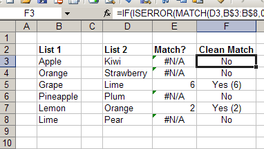
The figure above shows a spreadsheet with two lists (List 1 & List 2). The formula for cell E3 in the Match? column is =MATCH(D3,B$3:B$8,0). This tells Excel to lookup the value in D3 (Kiwi) and check to see if it is in List 1 which goes from B3 to B8. In this case it doesn't find a match so it returns #N/A. However, in this example it does find two matches, Lime and Orange at positions 6 and 2 in the list. The formula in cell E5 is =MATCH(D5,B$3:B$8,0) which does find a match and returns a 6.

Note: Make sure you include the $ when specifying the list to look in, in this case B$3:B$8. This will keep Excel from automatically changing the list when you copy and paste the formula to find the other values in List 2.

Clean it up (Optional)

You'll notice in column F under Clean Match it says No if it didn't find a match, and Yes with the position in brackets if it did find a match. To do this you can use the IF and ISERROR function along with MATCH to make it a little cleaner. The formula in cell F3 looks like this: =IF(ISERROR(MATCH(D3,B$3:B$8,0)),"No","Yes (" & MATCH(D3,B$3:B$8,0) & ")"). It's a little longer and more complicated but if we break it down you'll see what is happening. The IF function has 3 parts:

1. What you want to check
2. What to do if it's True
3. What to do if it's False.

In this case we're checking if ISERROR(MATCH(D3,B$3:B$8,0)) is True or False. We already know what the MATCH function does, and the ISERROR function just checks to see if the MATCH function returns an error (i.e. no match) or a number. If MATCH returns #N/A then ISERROR will be True, otherwise it will be False.

Now, if ISERROR is True (i.e. we didn't find a match) then the IF function will return the value "No". If ISERROR is False (i.e. we found a match) then the IF function will return the value "Yes (" & MATCH(D3,B$3:B$8,0) & ")". This is just the text Yes ( and then we get the position of the lookup value using the MATCH function and close it off with more text, in this case " )", and this is why we got the value Yes(6) when looking for Lime in list 1.

It isn't necessary to do this but sometimes it looks a lot nicer to have a specific result when you find or don't find a match.